
Free locomotion test
Overview
The initiative for the free locomotion test is to observe the motion of the prototype in an isolated environment free of external disturbances to confirm that the movement of the prototype is solely due to propulsion of the actuators. The motion of the prototype was captured by a high-definition camera and the displacement of the prototype was analyzed by a motion-tracking freeware, Kinovea. The test was conducted 3 times in a row using the same battery, with all the actuation conditions maintained the same to ensure comparative results. The best locomotion result was a forward displacement of 8 cm attained in 15 minute. The velocity, acceleration, and net propulsive force acting on the robot were calculated based on the robot's displacements using self-written MATLAB program. By analyzing the velocity, acceleration, and angle of turning of the robot, it appeared that the 6 actuators successfully propelled the robot forward. However, the mass of the robot has to be further reduced in order to amplify the velocity and acceleration.
This page includes the detailed procedures and analysis of the free locomotion test.
Procedures
The motion test setup is shown in Figure 5-1. The prototype was placed steadily into a tank filled with 5cm depth 1 M NaOH solution. Graph paper was placed at the bottom of the tank to serve as reference for robot's movements. A polycarbonate plastic board was used to cover tank to prevent disturbance of external air flow. A high-resolution camera (1920 x 1080, 25 fps) was placed on top of the polycarbonate board to record the robot's motion. The prototype was left to rest in the tank for 5-10 minutes the to let the initial disturbance settle down. Afterwards, the actuation of actuators are switched on by pressing the power button on the TV remote control. The motion of the prototype was then recorded until the actuation stopped due to exhaustion of battery power.


The recorded motion videos were analyzed using a motion tracking software, Kinovea. The movement of the robot is equivalent to the change in coordinate of an arbitrary point on the robot as shown in Figure 5-2. The (x,y) coordinate of the tracked point was captured every 0.4 second and saved as the units of pixels in an Excel file. Image pixel is converted to SI unit (centimeter) by dividing the number of pixels equal to 2 cm (the length of 1 square block) on the graph paper. This conversion constant should remain the same for different actuation test videos since the distance between the camera lens to the surface of electrolyte was maintained the same in all experiments. An example of the path traced out by the robot is re-plotted in MATLAB and shown in Figure 5-3.
Small ripples were identified in Figure 4-3 (a). It was difficult to determine whether the ripples were due to tracking error of the software or due to other disturbance, such as the unsteady movements of the robot or tank vibration. Hence, the small ripples were filtered out by curve fitting. All paths were fitted with a 10 order polynomial to form a smooth curve with the same trend of motion. The velocity and acceleration of the prototype were then calculated from the filtered displacement curve based on the method of difference. For example, the velocity and acceleration corresponding to a displacement in Figure 5-2 (b) are Figure 5-4 (c) and (d) respectively.

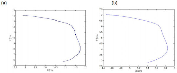
Figure 5-3. (a) The original and (b) filtered path traced out by an arbitrary point on the robot, and (c) the velocity and (d) acceleration calculated from the first- and second-derivative of the displacement of the robot respectively
Figure 5-2. Illustration of the point of origin and the tracking point in the motion-tracking software, Kinovea
Figure 5-1. Experimental setup of free locomotion test
The net propulsive force the experienced by the prototype was then determined by Newton’s second law: F = ma Where m = 50 g.
Assumptions
The following assumptions were made during the analysis of the experiments:
1. After resting in the tank for 5 minutes, the prototype was assumed to be at a stationary initial state.
2. During course of motion, the air movement and water current did not interfere with prototype's motion or the interference was negligible. Since the testing tank was not infinitely large, the air movement was negligible as the tank was sealed by a plastic cover on the top. after placing a cover on top of the tank. The electrolyte was as stationary as the prototype when the prototype's movements first started. Hence, the prototype's movement can be solely attributed to the actuators' propulsion or other disturbance sources resulted from the motion of the prototype.
3. All actuators functioned properly and did not deteriorate over time. The actuators' quality were assumed consistent over the testing period (~20 min) as the actuators can endure millions of actuation cycles before failure.
4. The prototype motion was captured by the camera at a filming angle that was perpendicular to the liquid surface. As the plastic cover was rigid enough to support the weight of the camera on the top without significant bending, the video taken would not include significant distortions.
Results
The results of the 3 motion test trials are shown below. Each set of photos display the initial and final positions of the robot during the motion test, as well as the path traced out by a point on the robot, and the net forces acting on the robot over time. The net force experienced by the robot was calculated by Newton's second law. The mass used in the calculation is 50g (as weighed), and the acceleration was obtained from taking the second derivative of displacement with respect to time.
Result analysis
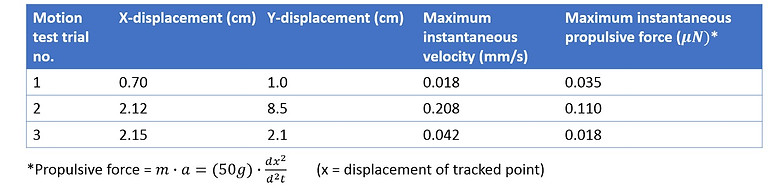
From Table 5-1, it appears that only motion test trial 2 yielded representative results. In trial 1, the displacement of the robot was equal to or less than 1 cm in both axis over 20 minutes. Whether the subtle movements of the robot was due to actuators' propulsion is in question. Some other factors such as worktable vibration might had also caused the subtle displacement.
In trial 3 we observed a displacement more significant than trial 1, but the robot moved at a very slow speed (0.042mm/s), which was not comparable to that of trial 2 (0.208 mm/s). Despite the fact that we had only one successful results in three trials, we could not conclude that propulsion by nickel hydroxide/oxyhydroxide actuators was unsuccessful, since in the second trial, the robot displaced approximately 10 cm along the thrust direction in a nearly disturbance-free environment. Any random object placed in the tank would not have moved this far without any help. Hence, we will take a closer look at the motion test result during second trial.
(i) Force analysis
The graph below plots the velocity and the force during trial 2 against time axis. It could be seen that the velocity was initially zero, but increased sharply together with the force from 0 ~ 14 sec. After the force reached a maximum at 14 second, the velocity continued to increase up to 0.208 mm/s at 28 sec. Subsequently, the force dropped dramatically, and the decline in velocity followed. These findings align with Newton's law of motion since force must result in changes in acceleration, which would be reflected on the velocity with some time delay.
Figure 5-7. Velocity and net propulsion force of the robot in second trial of motion test
We can take a further step to analyze the forces acting on the prototype. The net force should theoretically be equal to
F = (Actuators' propulsive force) - (body drag)- (surface tension) = ma
Note the following facts: Firstly, from drag formula, we know that the body drag is proportional to the square of the robot's velocity. Since the robot was moving at a very low velocity, the line and angle of contact the robot with the electrolyte remain relatively unchanged, and hence we assume that the surface tension acting on the robot as resistance was equal to some unknown constant. We can have the following hypothesis for the 'sequence' of forces that was taking effect during the motion test:
The velocity was initially zero, and so was the drag. The net force acting on the robot included actuators' propulsive force subtracted by some unknown value of surface tension. Since there was no drag, the initial acceleration could be high, and theoretically it should reach the maximum same as the 'net force acting on the robot' at t = 14 sec. As the robot accelerated, the velocity increased up to a certain value and peaked at t = 28 sec. Meanwhile, the hydrodynamic drag increased parabolically with the velocity. At some point of time, the drag caught up with the 'net' actuators' propulsive force (which is equal to actuators' propulsion subtracted by constant surface tension) and these two forces added together results in a near 'zero' net force, resulting in a velocity plateau (t = 40 sec ~ 80 sec, as shown in the indent of Figure 5-7). However, the net propulsive force of the actuators began to decrease over time (due to the decreasing battery power), and this result in reduction in the net force. At this instant, the hydrodynamic body drag became larger than the net actuator propulsive force from which point a negative acceleration was developed. This gave rise to the decrease in velocity, followed by a decrease in hydrodynamic body drag. Ultimately, the propulsive force, body drag, and robot's velocity all died down to zero.
(Noticed that negative 'net' force did not appear in Figure 5-7 because the force shown here was the square-root of sum of square of the propulsive force in both x- and y-direction. Namely, it is a product that will always remain positive. However, if we show the individual force in x- or y - direction, negative values will pop up)
The above hypothesis on the force sequence is illustrated with the graph below.

Motion test trial 1
The robot moved ~0.7 cm to the left on the x-axis and ~ 1 cm upward in the y-axis in 15 minutes. The small vibrations in the path traced out by the software were due to the unsteadiness of the tracking cursor, and was eliminated by curve-fitting in MATLAB. The net force acting on the robot approached a maximum value of 0.035 μN after the motion started for 14 seconds. It could be seen that after the initial peak, the force dropped to nearly zero. With zero net force, the robot maintained a constant speed accordingly at 0.018 mm/s from 70 sec ~ 550 sec. (velocity graph not shown here). The sudden rise in force at the end of the motion test was due to manual interference and is negligible.
Motion test trial 2

Direction of motion
The robot moved ~2.12 cm to the left on the x-axis and ~ 8.5 cm upward in the y-axis in 15 minutes. The major displacement was in the thrust direction (along y-axis), implying that the actuators might be able to propel. It could be observed from the path traced out by the robot that the significant displacement was mainly in the y-axis during the middle of the motion test, but during the beginning or at the end of the motion test, the robot mainly drifted in x-direction. The drifting to the left near the end of the motion test was due to unbalanced propulsive force when the left actuator at the front broke down. Simultaneously, the robot rotated 18 degrees clockwise. The net force reached a maximum after 14 seconds the motion test started with a value of 0.11 μN. After the initial peak, the force decreased continuously, most likely due to exhaustion of battery power. Likewise, the velocity first peaked at 0.208 mm/s after 14 seconds the test started, and then gradually dropped to zero throughout the motion test.
Direction of motion
Motion test trial 3

Direction of motion
The robot moved ~2.15 cm to the left in x-axis and ~ 2.1 cm upward in the y-axis. The net force acting on the robot first approached its maximum, 12 seconds after the locomotion test started, with a value 0.015 μN, and then peaked the second time at 80 seconds at 0.018 μN. After the two maxima, the force fluctuated at low amplitudes until the end of the motion test. The corresponding velocity profile (not shown here) shared a similar trend - it first peaked at 0.042mm/s after 12 seconds, and then gradually died down with some ups and downs.
The numerical results are summarized in the table below:
Table 5-1. Summary of key free locomotion test results

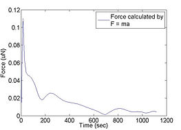
Figure 5-8. Schematic of different forces acting on the robot during the locomotion test
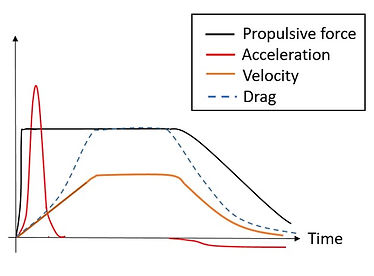
Note that the 'propulsive force' here refers to the net 'propulsive force' generated by the actuators (propulsive force subtracted by surface tension). Also, the 'net' force is not shown in this schematic, but it should be in proportional with acceleration (according to Newton's second law, F = ma). Finally, it was beyond our knowledge whether the propulsive force generated by the actuator was a constant or not before the battery started to fail. This was a part of the assumption adopted in the hypothesis in analyzing the force sequence. However, we observed that the net force in all three motion test trials peaked close to ~14 seconds after the tests started. This implies that the sum of actuator propulsive force and surface tension was very stable, so that the time to reach maximum acceleration could be consistent.
b. Estimated values of different forces
Given the analysis above, it is of scientific interest to estimate the propelling force of the actuators to facilitate a comparison with other types of actuators. We can also draw a comparison between force values estimated here, and calculated values using "drag-based approach" and "beam bending approach" as illustrated in "Material Characterization" page.
The force body diagram of the robot during the free locomotion test is shown below.
Figure 5-4. The photos of initial and final position of the robot during the first motion test (left 1,2), the path traced out by the robot (right 1), and the net force exerted on the robot estimated from the acceleration of the robot (right 2)
Figure 5-5. The photos of initial and final position of the robot during the second motion test (left 1,2), the path traced out by the robot (right 1), and the net force exerted on the robot estimated from the acceleration of the robot (right 2)
Figure 5-6. The photos of initial and final position of the robot during the third motion test (left 1,2), the path traced out by the robot (right 1), and the net force exerted on the robot estimated from the acceleration of the robot (right 2)
(ii) Error analysis
(a) External disturbance
Even though the prototype was put into the tank to situate for 5 minutes to let the disturbance settle down, the initial ‘stationary’ state was only observed from naked eyes and small vibrations may had been present. When the actuation was remotely started, it was not guaranteed that the prototype was at a perfect stationary state. The prototype might still be drifting due to any minor air movement or vibration nearby.
(b) Curve-fitting error
Curve-fitting function from MATLAB was applied on the traced path smooth out unwanted vibrations. Although each test contains more than 30,000 data points, overestimation and underestimation at some points may still arise due to this curve-fitting process. The values obtained may have a small percentage of error from the actual value.
(c) Parallax Error
The motion of prototype was captured by the camera placing on the transparent acrylic plate for analysis. The filming angle of the camera was assumed to be perpendicular to the solution surface in the motion test. However, since the weight of the camera will cause bending of the transparent acrylic plate so the video captured may not be at the level which was parallel to the liquid surface. In addition, the transparent acrylic plate may not be parallel to the liquid level inside the tank because the support on the plate by the walls of water tank may not be at the same level or the bench was not horizontal precisely. These causes parallax that the position and distance traveled of the prototype measured utilizing the test videos may deviates from the actual values. This measurement error led to lower accuracy of the result.
References:
[1] SODIUM HYDROXIDE: National Center for Biotechnology Information. (Retrieved Oct, 2017) https://pubchem.ncbi.nlm.nih.gov/compound/sodium_hydroxide#section=Physical-Description
[2] Cen L, & Erturk A, "Bio-inspired aquatic robotics by untethered piezohydroelastic actuation", Bioinspir. Biomim. Vol 8., pp 1 - 13, 2013.
Figure 5-9. Estimation of forces acting on the robot during motion
From the above estimation, we can see that the estimated actuation force by each actuator is 5.75mN, which is in the same order of magnitude as the piezoelectric tail actuator in the work by Cen and Erturk [2]. However, this is likely an overestimation, since we made use of maximum velocity to calculate the drag, and it is obvious from figure 5-7 that the velocity was not always a constant value as high as 0.208 mm/s. In addition, the calculation of surface tension here may be inaccurate since the surface energy density used is for a general salt solution. The interaction between styrofoam and sodium hydroxide was not considered when plugging in this value, and therefore the the calculated surface tension may not be realistic. We notice that the body drag and net propulsive force became negligible once surface tension was taken into account, and therefore the accuracy in the surface tension is a decisive factor whether the actuator's propulsion force is reasonably estimated. If we compare the actuation force obtained from current approach to the value from drag-based propulsion presented in the page of "Material Characterization", which gives an actuation force of ~ 17 µN per actuator, we notice a difference of nearly 3 order of magnitudes. Evidently, only one of them is correct. Therefore, further investigation is required.
